Mimic drilldown in a Microsoft Sentinel workbook

Overview

I recently saw a question about how to do a drilldown in a Microsoft Sentinel workbook. While Rod Trent wrote a post called How to Make Your Azure Sentinel Workbooks Even More Interactive with Drilldowns and Downloads – Azure Cloud & AI Domain Blog (azurecloudai.blog) about 2 years ago on this subject, it deals with exporting the data.

I was wondering if it would it be possible to do this inside of the workbook itself. The short version is “yes & no”. It is not possible to do a traditional drilldown inside a Microsoft Sentinel workbook, however you can mimic it. If you need a traditional drilldown, I suggest following Rod’s blog post and bring everything into Excel or recreate the report in something like PowerBI (and it just so happens, I have a series on how to do just that).

When I say you can mimic the drilldown functionality, I mean you can extract data from your bar or pie chart and use that elsewhere in the workbook. It is not an automatic process, unfortunately, so you will need to trigger the drilldown functionality.

Everything I do here should work with any workbook found in Azure, but I have only tested in Microsoft Sentinel.

The Workbook

I have saved the completed workbook at garybushey/AzureWorkbookDrilldown: This is an Azure Workbook that mimics a drilldown action (github.com) if you just want to upload it and play around. It is VERY basic but should give you all the information you need.

I started with the basic, out-of-the-box new Microsoft Sentinel workbook. I did modify the query for the bar chart only so I can see more than one entry in my environment and to have enough data to make it look interesting. The image below shows what the workbook looks like in edit mode. Each area will be discussed in more details below

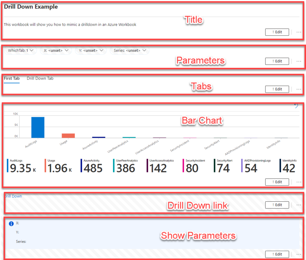
Title

This is just the title of the workbook. Nothing too fancy here.

Parameters

These are all the parameters that will be used. Each variable that will be used as the drilldown (X, Y, Series) and the tab (WhichTab) need to be defined here. The reason for the names of the “X”, “Y”, and “Series” variables will be explained below when we discuss the bar chart.

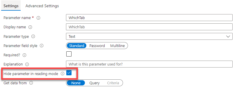
The image below shows the settings for the “WhichTab” parameter’s “Settings” tab, but ALL the parameters need to be set the same way. The only thing to note here is that the variable is hidden when not editting.

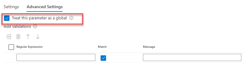
You will also need to go into the “Advanced Settings” tab and make sure the parameter is set as a global parameter as shown below. This ensures that the variable can be read throughout the workbook not matter where it is set.

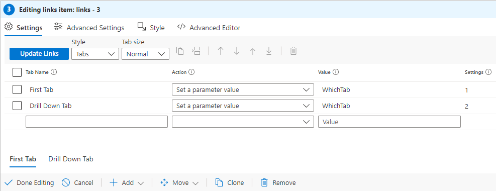
Tabs

Nothing to special here. Added a new “links/tabs” step, set the style to “Tabs” and filled out the rest as shown below.

Bar Chart

This is the out of the box bar chart that is created with a new workbook. As mentioned before, I did change the query to look back 30 days and to ignore the “ThreatIntelligenceIndicator” table only so I can see some useful data.

The big changes come in the “Advanced Settings” tab. Here is where you can set the variables to export. However, this does not work the same as it would if you were using a grid view. With a grid view, you select the name of the field to export, the name of the parameter, and so on.

However, with a chart, you cannot use the field names. You have to use the “x”, “y”, and “series” fields. If you mouse-over the information icon next to the “When items are selected, export parameters” checkbox, it will tell you this.

In the image below, you can see how I setup the “X” parameter. The rest are created using the same format. I am lazy so I just named the parameter as the same as the variable with the first letter capitalized.

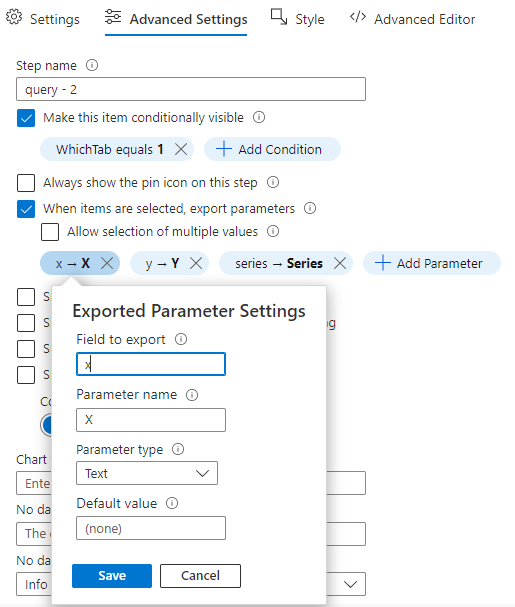
Also note that this step is hidden when we go to the second tab (when “WhichTab” equals 2).

Drill down link

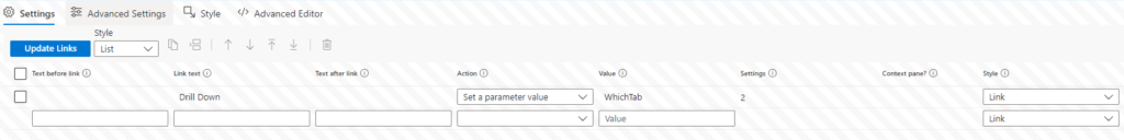
Now that we have the variables we need, we need to be able to trigger the drilldown. Sadly, this has to be done manually, using another link (or button).

The image below shows the basic configuration for this link. We want to set the “WhichTab” parameter, which is used to determine which tab to show. This is also hidden by default and more on that later. By setting the “WhichTab” parameter to 2, it will switch to the second tab (called “Drill Down Tab”)

We also need to go to the “Advanced Settings” tab and change when this link is visible. You can have it set to be visible whenever the first tab is visible, but I thought it would be better to only show when on the first tab and when you have selected a value to export. To do this, you have two different conditions. The first condition will show the link only when on the first tab and the second condition is to show the link only when the “X” parameter has a value (so only when you have selected a value). You can use any of the parameter for the second check so if you are using a pie chart rather than a bar chart, you would probably use the “Series” parameter.

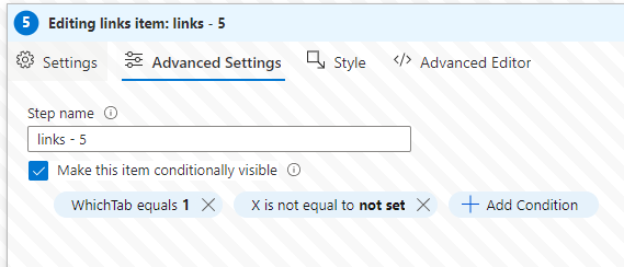
Figure 7 – Drill down link advanced settings

Show Parameters

This is just a text step that is used to show the various values to prove it is working. Nothing fancy here. It is just set to show only when on the second tab (i.e. “WhichTab” equals 2) and to show all the variables.

Summary

This blog post shows you how to sort of mimic the functionality of drilldowns in a Microsoft Sentinel workbook. It isn’t automatic like it is in other reporting products, but it works pretty well.