Introduction
Much of the investigative work done inside of Microsoft Sentinel, as well as many other Azure products that use KQL, deals with IP Addresses. Matching, comparing, and seeing if they show up in a table are many of the actions we perform against IP Addresses. Luckily, KQL provides many different functions to work with IP Addresses.
In this blog post we will look at them. While there are some IPv6 functions, we will not be looking into them as they work the same as IPv4 with the big difference being the IPv6 functions can work with IPV4 addresses while the IPv4 functions cannot work with IPv6 addresses.
We are going to assume you know about CIDR notation (referred to as IP Prefix in the KQL documentation). If not, there are a lot of websites that provide instruction about it as well as calculators.
ipv4_lookup
This command will perform a look up against a table to determine if the IP address passed in matches. This is the only command in this blog post that will work with tables, the others work with strings.
Since this is actually a plugin, it must be used in conjunction with the “evaluate” command as we will see below.
I am going to build on some of the examples shown in the KQL documentation for this command located at: ipv4_lookup plugin – Azure Data Explorer | Microsoft Docs. In this page, an external file is used that contains over 170,00 IP entries including information like content and country where the IP Address came from. Very useful for our testing purposes.
First, we will create a table that stores the information from this external data source. If you are not familiar with the “externaldata” command, you can find more information at: externaldata operator – Azure Data Explorer | Microsoft Docs
let IP_Data = externaldata(network:string,geoname_id:long,continent_code:string,continent_name:string ,country_iso_code:string,country_name:string,is_anonymous_proxy:bool,is_satellite_provider:bool)
    ['https://raw.githubusercontent.com/datasets/geoip2-ipv4/master/data/geoip2-ipv4.csv'];
Then we will create a dummy table of the IP Addresses we want to look at
let IPs = datatable(ip: string) [
    '2.20.183.12/25',   // United Kingdom
    '2.20.183.12/23',   // United Kingdom
    '5.8.1.2',       // Russia
    '192.165.12.17', // Sweden
    '192.168.1.1'
];
Now that we have the tables we want to use, we can start looking at how to use this command. The basic format for this command is
Table | evaluate ipv4_lookup(lookup_table, table column to lookup, lookup_table column to lookup, return_unmatched?In our case, we want to use “IPs” as the table and use the “ip” column to perform the lookup, “IP_Data” is the table we want to perform the lookup against, and “network” is the column that we will use in “IP_Data” to perform the lookup. We will discuss “return_unmatched” later. Our KQL will look like
IPs | evaluate ipv4_lookup(IP_Data, ip, network)This will return the data as shown below. Note that I don’t know how often that external file is updated so your results may look different

As you can see, the IP Addresses that match are shown. Couple of things to note here. First is that this command can expand the CIDR notation of the IP addresses to see if they match. The second is that the order of the parameters.
You first specify the lookup table, then the lookup column from the table you pass, and then the lookup column from the lookup table. Seems a bit out of order. One reason the parameters are in this order is because you can specify multiple columns from the lookup table to match upon. While in this example we only perform a lookup against the “network” column, we could also perform a lookup against the “continent_code”, “count_iso_code”, or any of the other columns, if we had data in our table that can be used to do the match.
It is worth pointing out that only the matches show up. While this may be what you want, especially in an analytic rule, there may be occasions when you want to see all the IP Addresses from the table you are using to perform the search. There is a parameter that can resolve this issue.
By adding the “return_umatched=true” parameter, you will see all the IP Address from the table you use to perform the search. Using the same tables, the command
IPs | evaluate ipv4_lookup(IP_Data, ip, network, return_unmatched = true)Will return
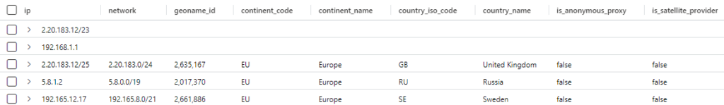
You can see that the first two entries don’t have any data from the lookup table being returned. This is because there is no match. This would be useful in a workbook where you want to see if any IP Addresses in your domain match against a table containing indictors of compromise. You will see the ones that have no indicators as well as those that do.
has_ipv4 / has_any_ipv4
These functions will return a value indicating whether one of specified IPv4 addresses appears in a text. The only difference between the two is that “has_any_ipv4” will allow multiple IP Addresses to be entered as a parameter to match against.
The format of these commands are
has_ipv4(string, IP_address1...IP_addressN)The following command will return true
print has_any_ipv4('05:04:54 127.0.0.1 GET /favicon.ico 404', '127.0.0.1', '127.0.0.2')You may be wondering why not just use a text matching function. I know I did. These commands do perform a bit more logic to determine whether something is a match or not. For instance, the following command will return false
print has_any_ipv4('05:04:54127.0.0.1 GET /favicon.ico 404', '127.0.0.1', '192.168.1.1')Did you see why? The IP Address in the string is not formatted correctly. There should be space between the “:54” and “127”. A regular string comparison will return true since the text is matched.
has_any_ipv4_prefix / has_ipv4_prefix
These commands will return a value indicating whether one of specified IPv4 address prefixes appears in a text. Seems to be the same as the above commands, right? Even the format of the commands are the same.
The big difference lies in the way that the IP Addresses to match can be entered. Using these commands, you do not need to enter the entire IP Address. The command below will return true:
print has_any_ipv4_prefix('05:04:54 127.0.0.1 GET /favicon.ico 404', '127.0.', '192.168.') Keep in mind that the IP Address to match against either has to be the full IP Address or end in a dot. The command below will return false (note the first IP Address to match against)
print has_any_ipv4_prefix('05:04:54 127.0.0.1 GET /favicon.ico 404', '127.0', '192.168.')I am sure you can see how useful these functions can be.
ipv4_compare / ipv6_compare
These functions compare two IPv4/v6 strings. The two IPv4/v6 strings are parsed and compared while accounting for the combined IP-prefix mask calculated from argument prefixes, and the optional prefix mask parameter.
Because you are doing a comparison rather than a match (described below), these functions return more than just true or false. They return
- 0: If the long representation of the first IPv4/v6 string argument is equal to the second IPv4/v6 string argument
- 1: If the long representation of the first IPv4/v6 string argument is greater than the second IPv4/v6 string argument
- -1: If the long representation of the first IPv4/v6 string argument is less than the second IPv4/v6 string argument
- null: If conversion for one of the two IPv4/v6 strings wasn’t successful
Let’s look at some examples that will hopefully help to understand these functions. In the example below, the “result” column will have “0” in it, in all cases
datatable(ip1_string: string, ip2_string: string) [
    '192.168.1.0', '192.168.1.0',           // Equal IPs
    '192.168.1.1/24', '192.168.1.255',     // 24 bit IP-prefix is used for comparison
    '192.168.1.1', '192.168.1.255/24',  // 24 bit IP-prefix is used for comparison
    '192.168.1.1/30', '192.168.1.255/24',  // 24 bit IP-prefix is used for comparison
]
| extend result = ipv4_compare(ip1_string, ip2_string)
I think the first entry is obvious, “192.168.1.0” equals itself. The second entry may take some examination to see why the two values are equal. “192.168.1.1/24” returns the IP ranges of “192.168.1.1” through “192.168.1.255”. Since we are comparing to “192.168.1.255”, which falls into the range, the values are equal.
The third entry is the same as the second entry, just reversed. “192.168.1.255/24” returns the same range as the second entry and since “192.168.1.1” is part of that range, they are considered to be equal.
In the last entry, “192.168.1.1/30” returns the IP range of “192.168.1.1” through “192.168.1.3”. We already know what “192.168.1.255/24” returns, and we can see that the first range falls inside the second range, so they are equal.
Let’s look at some more examples to see different values in the “result” column
datatable(ip1_string: string, ip2_string: string) [
    '192.168.1.0', '192.168.1.0',       // Equal IPs
    '192.168.0.1/24', '192.168.1.255',     // 24 bit IP-prefix is used for comparison
    '192.168.1.1', '192.168.1.255/30',  // 30 bit IP-prefix is used for comparison
    '192.168.1.0/23', '192.168.0.0',  // 23 bit IP-prefix is used for comparison
     '192.168.2.0/23', '192.168.0.0',  // 23 bit IP-prefix is used for comparison
]
| extend result = ipv4_compare(ip1_string, ip2_string)
In this case, the first entry is still equal so “result” contains “0”. In the second entry, “192.168.0.1/24” returns the range of “192.168.0.1” through “192.1680.255”. “192.168.1.255” does not fall into this range at all. In fact, “192.168.0.1/24” is considered to be less than “192.168.1.255” (see the “parse” commands below) so “result” will contain “-1”.
The third entry also has “-1” in the “result” column. In this case “192.168.1.255/30” returns “192.168.1.252” to “192.168.1.255”. Since “192.168.1.1” is less than that, “result” has “-1”
The fourth entry has “0” in the “result” column. “192.168.1.0/23” will actually return “192.168.0.0” through “192.168.1.255”. Since “192.168.0.0” falls into that range, “result” has a “0”.
Finally, the fifth entry will have a “1” in the “result” column. “192.168.2.0/23” yields “192.168.2.0” through “192.168.3.255”. The lowest entry in this range is greater than “192.168.0.0” so a “1” is stored in the “result” column.
ipv4_is_in_range / ipv4_is_in_any_range
These commands will check to see if IPv4 string address is in IPv4-prefix notation range. The “ipv4_is_in_any_range” will allow for multiple IP Addresses to check against.
This uses the same logic we discussed previous section to determine if an IP address falls into the range. The format of this command is
ipv4_is_in_range(ipAddress,IpRange,...IpRangeN)ipv4_is_match / ipv6_is_match
These functions determines if two IPv4/v6 strings match. The two IPv4/v6 strings are parsed and compared while accounting for the combined IP-prefix mask calculated from argument prefixes, and the optional Prefix mask argument.
These functions work just like “ipv4_compare” and “ipv4_compare” described above where the result equals “0”.
ipv4_is_private
This function will check to see if IPv4 string address belongs to a set of private network IPs. Basically, it will see if the IP Address passed in falls into one of these ranges:
- 10.0.0.0 – 10.255.255.255
- 172.16.0.0 – 172.31.255.255
- 192.68.0.0 – 192.168.255.255
ipv4_netmask_suffix
This function will the value of the IPv4 netmask suffix (AKA CIDR mask) from IPv4 string address. While this is easy to see by just looking at the IP Address, it is a bit harder for a computer to determine. Here are some examples to show you how this function works:
datatable(ip_string: string) [
    '10.1.2.3', '192.168.1.1/24', '127.0.0.1/16',
]
| extend cidr_suffix = ipv4_netmask_suffix(ip_string)
The result are:
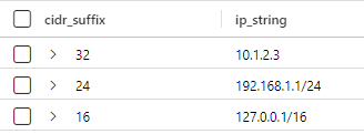
It should be pretty obvious why the values in “cidr_suffix” are there. (I also find it interesting that the documentation for this command refers to “IP-prefix notation” while the example calls it “cidr_suffix”). Note that a single IP address has the hidden suffix of “32” which yields just a single value.
parse_ipv4 / parse_ipv6
These functions convert a IPv4/v6 string to long (signed 64-bit) number representation in big-endian order. Don’t worry about the big-endian order, it just means that the numbers are processed before the last numbers (and the term can actually be traced back to Gulliver’s travels when two factions were fighting about whether to open an egg on the big end or the small end).
Here is an example of how to use this function
print parse_ipv4("127.0.0.1") == 2130706433parse_ipv4_mask / parse_ipv6_mask
These functions work just like the ones above, except that a CIDR mask can be included. An example of the command is
print parse_ipv4_mask("127.0.0.1", 24) == 2130706432You may notice that this number being returned is one less than in the example we showed above. That is because the first entry in “127.0.0.1/24” is “127.0.0.0” which is one less than “127.0.0.1”.
While you may not actually use these last two functions, they are used behind the scenes in other functions we have gone over and are quite useful.
Summary
We have gone over the KQL functions that are used when working with IP Addresses. With these functions, you can evaluate IP Addresses and will hopefully help you with your investigations.